Forest plots, survival curves, ROC curves.
These show up on roughly 15-20 INBDE questions. They look dense. Most candidates spend minimal time on them because the charts seem complicated—and because biostatistics feels low-yield compared to pharmacology or anatomy.
It's not. Each chart type answers one specific clinical question. Once you know that question, you know what to look for.
This post assumes you've covered Part 1: The Foundation (2x2 tables, box plots, scatter plots).
Forest Plots: "What Do All These Studies Say Together?"
Five studies examine whether implants or bridges have better long-term outcomes. Two favor implants. Two show no significant difference. One slightly favors bridges. What do you tell the patient?
This is exactly what a forest plot answers. It takes multiple studies on the same question and combines them into a single pooled estimate. This process is called meta-analysis—and it sits at the top of the evidence hierarchy because it doesn't depend on any single study being correct.
Before you can read the plot, you need to understand Odds Ratios (OR):
- OR = 1.0 → Both groups have the same odds (no difference)
- OR < 1.0 → The first group has lower odds (e.g., fewer failures)
- OR > 1.0 → The first group has higher odds (e.g., more failures)
Here's how to read the plot itself:
- Each horizontal line = one study's result. The square in the middle is that study's estimate. The line extending left and right shows the confidence interval—the range where the true value probably falls. A wider line means more uncertainty.
- The vertical line down the middle (at 1.0) = "no difference between groups." If a study's horizontal line crosses this vertical line, that study alone didn't find a statistically significant difference.
- The diamond at the bottom = the combined result of all studies pooled together. If the diamond doesn't touch the middle line, the overall finding is statistically significant.
One more number to know: I² (I-squared) tells you whether the studies agree with each other:
- I² below 50% = studies found similar results (good)
- I² above 50% = studies are contradicting each other (interpret with caution)
The following forest plot compares implant failure rates to fixed partial dentures across five trials:
A systematic review compares failure rates between dental implants and fixed partial dentures (FPDs) across five clinical trials.
Forest plot cheat sheet:
- Diamond doesn't cross the line → Statistically significant overall
- Diamond crosses the line → No significant difference
- I² < 50% → Studies agree (results are reliable)
- I² > 50% → Studies conflict (interpret with caution)
- Bigger squares = larger studies (weighted more heavily)
Where students get tripped up:
-
Confusing individual studies with the pooled result. A question might ask "Is there a significant difference?" Students see that most individual studies cross the null line and answer "no." But the diamond (pooled result) doesn't cross—so the overall answer is "yes, significant."
-
Forgetting what side favors what. Always check the labels. "Favors Treatment" on the left means OR < 1 is good for treatment. Some plots flip this. Read the axis labels before answering.
-
Ignoring I². A pooled result might look impressive (OR = 0.3, p < 0.001), but if I² = 85%, the studies are contradicting each other. The INBDE will ask whether you should trust results with high heterogeneity.
Survival Curves: "How Long Until It Fails?"
A patient asks: "How long will this implant last?"
You can't give a single number because different patients fail at different times. Some implants fail at 6 months. Some last 20 years. What you need is a way to show the probability of survival over time—and that's exactly what a survival curve does.
How to read a survival curve:
-
Start at the top left. The curve begins at 100% (or 1.0)—everyone starts "alive" or with their restoration intact.
-
Follow the steps down. Each drop represents an event (failure, death, recurrence). The curve is stepped, not smooth, because events happen at specific time points.
-
Compare heights at any time point. If you want to know "What percentage survived to 5 years?", find 5 years on the x-axis and read the y-value. Higher = better.
-
Compare two curves. The curve that stays higher longer is the better treatment. If curves cross, interpretation gets complicated—early advantage might reverse over time.
The statistical test: Log-rank test
This compares two survival curves and gives you a p-value:
- p < 0.05 → The curves are significantly different
- p ≥ 0.05 → Any difference could be random chance
Hazard Ratio (HR) quantifies how much better one treatment is:
- HR = 1.0 → No difference in risk
- HR = 2.0 → Twice the risk of failure
- HR = 0.5 → Half the risk of failure
If the 95% CI for HR includes 1.0, the difference isn't statistically significant—same rule as confidence intervals everywhere else.
A 5-year prospective study compares implant survival between immediate and delayed placement protocols.
Why not just report "X% survived at 5 years"? Because patients drop out. Some move away. Some die of unrelated causes. Some are still being followed when the study ends. These are called censored observations—we know the patient hadn't failed yet, but we don't know their final outcome. Survival analysis handles censoring properly; a simple percentage would either ignore these patients or miscount them.
Survival curve cheat sheet:
- Higher curve = better survival
- Steeper drop = more failures at that time
- Log-rank p < 0.05 = curves are significantly different
- HR < 1 = reduced risk (treatment is protective)
- HR > 1 = increased risk
- HR CI includes 1.0 = not significant
Where students get tripped up:
-
Mixing up "survival" with "alive." In dental contexts, "survival" usually means the restoration is still functional—not that the patient is living. An implant "survives" if it hasn't failed, even if the patient died of something unrelated.
-
Forgetting to check the p-value. Two curves can look different visually but have p = 0.4. The INBDE will show curves that appear separated and ask if the difference is significant. Always check the log-rank test result.
-
Confusing HR direction. HR = 0.5 means half the risk—that's good if the outcome is failure. Students sometimes think lower HR is worse because the number is smaller.
ROC Curves: "Which Test Is Better?"
You have two salivary biomarkers that might detect oral cancer. Both give you a number. How do you decide which one to use clinically?
You could pick a cutoff and calculate sensitivity and specificity for each test. But that only tells you how they perform at that specific cutoff. What if a different cutoff would be better? An ROC curve shows you how each test performs at every possible cutoff—so you can compare their overall diagnostic ability.
How to read an ROC curve:
-
Understand the axes. The y-axis is sensitivity (true positive rate). The x-axis is 1-Specificity (false positive rate). Yes, the x-axis is confusing—it's "1 minus specificity," not specificity itself.
-
The diagonal line is worthless. A test that falls on the diagonal from bottom-left to top-right has AUC = 0.5. It's no better than flipping a coin.
-
Upper-left corner is perfect. A perfect test would be a single point at (0, 1)—100% sensitivity, 0% false positives. Real tests form curves that bow toward this corner.
-
The curve that bows more wins. If Test A's curve is always above Test B's curve, Test A is better at every threshold.
Area Under the Curve (AUC) summarizes overall performance in one number:
| AUC | Interpretation |
|---|---|
| 0.9 - 1.0 | Excellent |
| 0.8 - 0.9 | Good |
| 0.7 - 0.8 | Fair |
| 0.5 | Useless (coin flip) |
Researchers compare two salivary biomarkers for early oral cancer detection against histological diagnosis.
Comparison of Salivary Biomarkers for Oral Cancer Detection
ROC curve cheat sheet:
- Curve hugging upper-left = better test
- AUC closer to 1.0 = better discrimination
- AUC = 0.5 = worthless (coin flip)
- Moving up the curve = higher sensitivity, more false positives
- Moving down the curve = higher specificity, more missed cases
Where students get tripped up:
-
The x-axis confusion. It's 1-Specificity, not Specificity. So when x = 0.2, specificity is 80% (not 20%). The INBDE loves asking "What is the specificity at point X?" and giving 1-Specificity as a wrong answer.
-
Thinking AUC changes with threshold. AUC is a property of the test itself. Changing your cutoff moves you along the curve—it doesn't change the curve or its AUC.
-
Forgetting the clinical context. A question might ask which cutoff to use for cancer screening. The answer should favor high sensitivity (catch all cancers) even if specificity suffers. For confirmatory testing, you'd want the opposite.
The clinical insight: Moving along the curve always involves a tradeoff. You can't maximize both sensitivity and specificity—you have to choose based on the clinical situation.
- Screening test? Prioritize sensitivity. Missing cancer is worse than extra biopsies.
- Confirmatory test? Prioritize specificity. Don't tell healthy people they have cancer.
Summary
Forest plots: Look at the diamond. If it doesn't cross the null line (1.0 for ratios), the pooled result is significant. Check I² for whether studies agree.
Survival curves: Higher curve = better survival. Log-rank test tells you if the difference is significant. HR < 1 means reduced risk.
ROC curves: Curve hugging upper-left wins. AUC closer to 1.0 = better test. Remember: x-axis is 1-Specificity, not Specificity.
The Concepts Without Charts
About a third of biostatistics questions don't include any visual. They test concepts directly:
- A p-value of 0.08: significant or not?
- Confidence interval includes 1.0: what does that tell you?
- Type I vs Type II error: which is which?
- Cohort study vs RCT: which proves causation?
Part 3 covers these four concepts with the same approach—what the INBDE actually asks, and the traps it sets.
Part 3: Concepts Without Charts →
Sources: